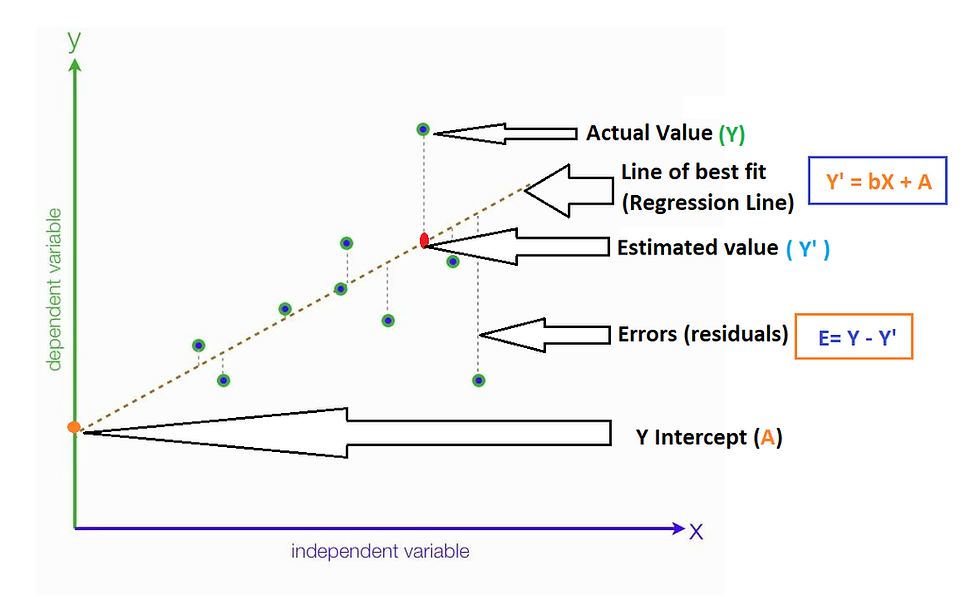
Linear Regression is one of the most fundamental techniques in data science and statistics. It’s widely used to model and analyze the relationship between a dependent variable and one or more independent variables. In this blog post, we’ll dive into the theory behind Linear Regression, the mathematical principles that drive it, and an end-to-end Python example to illustrate how it works.
Table of Contents
ToggleWhat is Linear Regression?
Linear Regression is a statistical method used to understand the relationship between variables. Specifically, it attempts to model the relationship between a dependent variable Y and one or more independent variables X. The goal is to predict the dependent variable using the independent variables.
Simple Linear Regression
Simple Linear Regression involves a single independent variable and aims to find the best-fitting line through the data points. The relationship is modeled by a linear equation:
Y=β0+β1X+ϵ
Where:
- Y is the dependent variable.
- X is the independent variable.
- β0 is the intercept of the line.
- β1 is the slope of the line.
- ϵ is the error term, capturing the difference between observed and predicted values.
What is the Best Fit Line?
The “Best Fit Line” is the line that minimizes the difference between the actual data points and the predicted values from the model. This line is found by minimizing the sum of the squared differences (errors) between the observed values and the values predicted by the model.
Mathematically, the Best Fit Line minimizes the following cost function:

where yi is the actual value, and 𝛽0 + 𝛽1𝑥i is the predicted value.
Cost Function for Linear Regression
The Cost Function measures how well the model predicts the dependent variable. For Linear Regression, the Cost Function used is the Sum of Squared Errors (SSE) or Residual Sum of Squares (RSS):

The goal is to find the values of β0 and β1 that minimize this cost function, ensuring the line fits the data as well as possible.
Gradient Descent for Linear Regression
Gradient Descent is an optimization algorithm used to find the minimum of a function. For Linear Regression, it helps find the optimal values of β0 and β1 that minimize the Cost Function.
Here’s how Gradient Descent works:
- Initialize the parameters β0 and β1 with some initial values.
- Compute the gradient (partial derivatives) of the Cost Function with respect to β0 and β1.
- Update the parameters in the direction that reduces the Cost Function. The update rule is:

where α is the learning rate.
4. Repeat steps 2 and 3 until convergence, i.e., when the parameters stop changing significantly.
Why is Linear Regression Important?
Linear Regression is important for several reasons:
- Simplicity: It’s easy to understand and implement, making it a good starting point for predictive modeling.
- Interpretability: The coefficients β0β1 are straightforward to interpret, providing insights into the relationship between variables.
- Efficiency: It’s computationally efficient and can be used with large datasets.
- Foundation for Complex Models: It forms the basis for more complex regression models, such as polynomial and multiple regression.
Evaluation Metrics for Linear Regression
To assess the performance of a Linear Regression model, several evaluation metrics are used:
a. Coefficient of Determination (R-Squared, R^2)
The Coefficient of Determination measures how well the model explains the variability of the dependent variable. It’s calculated as:

- where SST (Total Sum of Squares) is:
- In SST yˉ is the mean of the actual values.
An R2 value closer to 1 indicates a better fit, meaning the model explains a high proportion of the variability in the dependent variable.
b. Root Mean Squared Error (RMSE)
The Root Mean Squared Error measures the average magnitude of the prediction errors. It’s the square root of the average of the squared errors:

where y^i are the predicted values. Lower RMSE values indicate better model performance.
Assumptions of Linear Regression
Linear Regression relies on several key assumptions:
- Linearity: The relationship between the dependent and independent variables is linear.
- Independence: The residuals (errors) are independent.
- Homoscedasticity: The residuals have constant variance.
- Normality: The residuals are normally distributed.
Violations of these assumptions can lead to biased or inefficient estimates.
Hypothesis in Linear Regression
In Linear Regression, the hypothesis is the model that predicts the dependent variable based on the independent variables:
h(X) = β0+β1X
where h(X) is the hypothesis function (or the prediction).
Assessing the Model Fit
To assess how well the model fits the data:
- Visualize: Plot the data points and the regression line to visually inspect the fit.
- Check Metrics: Evaluate R2 and RMSE to quantify model performance.
- Residual Analysis: Examine residual plots to ensure assumptions are met and identify any patterns not captured by the model.
Practical Example: Linear Regression in Python
Step 1: Generating Synthetic Data
We’ll start by creating a dataset with a linear relationship plus some random noise.
import numpy as np
import pandas as pd
import matplotlib.pyplot as plt

# Generating synthetic data
np.random.seed(0)
X = 2 * np.random.rand(100, 1)
y = 4 + 3 * X + np.random.randn(100, 1)

# Convert to DataFrame for ease of use
data = pd.DataFrame(np.hstack((X, y)), columns=['X', 'y'])
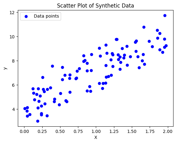
Step 2: Visualizing the Data
Visualizing the data helps us understand its distribution and the relationship between the variables.
plt.scatter(X, y, color='blue', label='Data points')
plt.xlabel('X')
plt.ylabel('y')
plt.title('Scatter Plot of Synthetic Data')
plt.legend()
plt.show()
Step 3: Fitting the Linear Regression Model
We’ll use the LinearRegression class from sklearn to fit our model.
from sklearn.linear_model import LinearRegression

# Create and fit the model
model = LinearRegression()
model.fit(X, y)

# Get the parameters
beta_0 = model.intercept_[0]
beta_1 = model.coef_[0][0]

print(f"Intercept (β0): {beta_0}")
print(f"Slope (β1): {beta_1}")
Below are the Slope & Intercept values.
- Intercept (β0): 4.222151077447231
Slope (β1): 2.968467510701019
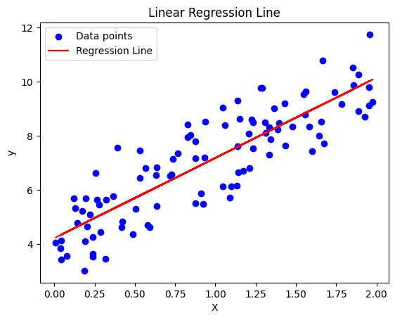
Step 4: Predicting and Plotting the Regression Line
Finally, we’ll use the model to make predictions and plot the regression line.
# Predict values
y_pred = model.predict(X)

# Plot the data and the regression line
plt.scatter(X, y, color='blue', label='Data points')
plt.plot(X, y_pred, color='red', label='Regression Line')
plt.xlabel('X')
plt.ylabel('y')
plt.title('Linear Regression Line')
plt.legend()
plt.show()
Step 5: Evaluating the Model
We’ll calculate the Mean Squared Error (MSE) to evaluate the performance of our model.
from sklearn.metrics import mean_squared_error

# Calculate and display Mean Squared Error
mse = mean_squared_error(y, y_pred)
print(f"Mean Squared Error: {mse}")
- Mean Squared Error: 0.9924386487246479
The MSE value provides a measure of how well our model’s predictions align with the actual values. Here’s what you need to consider:
- Magnitude: The MSE value of approximately 0.992 indicates the average squared deviation between the predicted and actual values. A lower MSE generally signifies a better model fit.
- Context: The absolute value of MSE is dependent on the scale of the data. For different datasets or problems, what constitutes a “good” MSE can vary. It’s important to compare the MSE to baseline models or other benchmarks to assess the performance meaningfully.
- Comparison: When evaluating model performance, it’s helpful to compare the MSE against the MSE of other models or different configurations. This comparison can provide insight into whether our model is performing well or if there’s room for improvement.
Conclusion
Linear Regression is a foundational technique in both statistics and machine learning. By understanding the theory, mathematics, and evaluation metrics, you can effectively apply Linear Regression to various problems, from simple predictive tasks to more complex analyses.
To practice and enhance your skills, consider working with real-world datasets. For example, you can explore the Boston Housing Dataset on Kaggle. This dataset offers a great opportunity to apply your Linear Regression knowledge, from data preprocessing to model evaluation. Engaging with such datasets will help solidify your understanding and improve your practical skills in Linear Regression.


