Understanding Dispersion of Data: 4 Key Metrics Explained

When analyzing data, knowing just the average (mean) doesn’t give us a complete picture. To truly understand the data, we need to measure how spread out or varied the data points are. This is where measures of dispersion come in. They help us understand the variability within a dataset. We’ll explore several key measures of dispersion, explain each concept in detail, and use simple examples to illustrate them.

For a comprehensive understanding of central tendency and dispersion together, explore our previous article on Measures of Central Tendency.

1. What is Dispersion of Data?

Dispersion of data refers to how spread out the values in a dataset are. It provides insight into the variability and consistency of the data. While measures of central tendency like the mean give us an idea of the average value, dispersion metrics help us understand how much the values deviate from this central point.

Why Do We Need Measures of Dispersion?

1. Understanding Variability: Measures of dispersion provide insights into how much the data values deviate from the average. This is essential because datasets with the same mean can have very different spreads. For instance, two datasets might both have an average score of 75, but if one has scores clustered closely around 75 and the other has scores spread out over a wide range, they represent different levels of consistency and reliability.
2. Identifying Outliers: Measures of dispersion help in identifying outliers or anomalies in the data. For instance, if most of the data points are tightly packed but there are a few significantly different values, these outliers will affect measures like the range and standard deviation.
3. Making Comparisons: When comparing datasets, measures of dispersion allow us to assess which dataset has more variability. This is useful in various fields such as quality control, finance, and research, where understanding consistency or variability is crucial.
4. Risk Assessment: In finance, measures of dispersion like standard deviation are used to assess the risk or volatility of investments. A high standard deviation indicates higher risk due to greater variability in returns.
5. Data Interpretation: Measures of dispersion aid in interpreting data more effectively by providing a clearer picture of the distribution and spread of data points around the central value.

How Can We Use Measures of Dispersion in Our Data?

1. Descriptive Analysis: Use measures of dispersion to summarize and describe the main features of a dataset. This helps in gaining an initial understanding of the data’s distribution.
2. Quality Control: In manufacturing and production, measures of dispersion can be used to monitor the consistency of products. For instance, if the thickness of a material is supposed to be uniform, measures of dispersion can help identify variations.
3. Statistical Inference: In hypothesis testing and statistical modeling, understanding dispersion helps in making inferences about the population from a sample. Measures like standard deviation are used in confidence intervals and significance tests.
4. Decision Making: Businesses use measures of dispersion to make informed decisions. For example, in sales forecasting, understanding the variability in sales figures helps in setting realistic targets and preparing for potential fluctuations.
5. Benchmarking: Organizations use measures of dispersion to compare performance against benchmarks or competitors. For example, comparing the variability in customer satisfaction scores across different departments or stores.

2. Types of Measures of Dispersion

Range

Range is the simplest measure of dispersion. It tells us the extent of the spread between the maximum and minimum values in a dataset.

Formula: Range= Maximum value − Minimum value

Example: Consider the test scores: 60, 75, 80, 85, and 90.

• Maximum value = 90
• Minimum value = 60

So, the range is: Range= 90 − 60 = 30

This means the scores are spread over a range of 30 points.

Variance

Variance measures the average squared deviation of each data point from the mean. It tells us how much the data points differ from the average value.

Population variance

Sample variance 

Observation near to mean value gets the lower result and far from means gets higher value.

Where:

• xi​ = each individual value
• μ = population mean
• xˉ= sample mean
• N = number of values in the population
• n = number of values in the sample

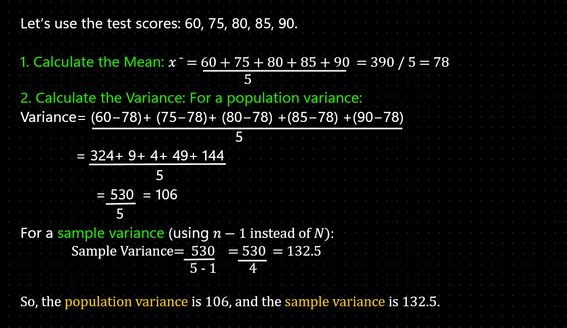
Example Calculation:

• Population Variance (106): This is the measure of how data points in the entire population deviate from the population mean. It represents the average squared deviation from the mean for every data point in the population.
• Sample Variance (132.5): This is the measure of how data points in a sample (a subset of the population) deviate from the sample mean. It’s calculated using $n-1$ (where $n$ is the sample size) in the denominator to correct for the bias in the sample’s estimate of the population variance.

Standard Deviation

Standard Deviation is the square root of the variance. It provides a more intuitive measure of dispersion because it’s in the same unit as the original data.

• 68 % of values lie within 1 standard deviation.
• 95 % of values lies within 2 standard deviation.
• 99.7 % of values lie within 3 standard deviation.

Formula: Standard Deviation = √Variance

Example Calculation:

• Using the population variance (106): Standard Deviation = √106 ≈ 10.30
• Using the sample variance (132.5): Standard Deviation = √132.5 ≈ 11.52

So, the standard deviation for the population is approximately 10.30, and for the sample, it is approximately 11.52.

Spread and Variability

• Population Standard Deviation (10.30): Indicates that, on average, data points in the entire population deviate from the mean by approximately 10.30 units. This gives a sense of the typical distance between individual values and the population mean.
• Sample Standard Deviation (11.52): Shows that the data points in the sample deviate from the sample mean by about 11.52 units on average. The sample standard deviation is generally larger than the population standard deviation due to the adjustment factor used in its calculation. Visit here to Visual the Standard Deviation

Quantiles are values that divide a dataset into equal-sized intervals. The most commonly used quantiles are the quartiles.

• First Quartile (Q1): The 25th percentile. It’s the value below which 25% of the data falls.
• Second Quartile (Q2): The 50th percentile (median). It’s the middle value of the dataset.
• Third Quartile (Q3): The 75th percentile. It’s the value below which 75% of the data falls.

Interquartile Range (IQR) measures the range within which the central 50% of the data lies.

Formula: IQR= Q3 − Q1

So the IQR we calculate based upon the Five Number Summary. It is a set of descriptive statistics that provides a quick overview of the distribution of a dataset. It includes:

1. Minimum: The smallest value in the dataset.
2. First Quartile (Q1): The 25th percentile, which is the median of the first half of the data.
3. Median (Q2): The 50th percentile, or the middle value when the data is ordered.
4. Third Quartile (Q3): The 75th percentile, which is the median of the second half of the data.
5. Maximum: The largest value in the dataset.

Calculate the IQR Using the Five Number Summary

1. Sort the Data: Arrange your data in ascending order.

2. Determine the Five Number Summary:

• Minimum: The smallest data value.
• Q1: The median of the first half of the data (excluding the median if the number of data points is odd).
• Median (Q2): The middle value of the data.
• Q3: The median of the second half of the data.
• Maximum: The largest data value.

3. Calculate the IQR:

$$\text{IQR}=Q3-Q1$$

Solved Example

Dataset: 5, 7, 8, 12, 15, 18, 21, 25, 28, 30

1. Sort the Data: (Already sorted in this case)

2. Calculate the Five Number Summary:

• • Minimum: 5
  • Median (Q2): The middle value. With 10 data points, the median is the average of the 5th and 6th values.

1. • First Quartile (Q1): The median of the first half of the data (5, 7, 8, 12, 15). The median of this subset is 8.
   • Third Quartile (Q3): The median of the second half of the data (18, 21, 25, 28, 30). The median of this subset is 25.
   • Maximum: 30

3. Calculate the IQR:

IQR= Q3 − Q1 = 25 − 8 =17

So, the Interquartile Range (IQR) of 17 means that the central 50% of the data values fall within a range of 17 units. In our dataset, this range extends from the 25th percentile (Q1 = 8) to the 75th percentile (Q3 = 25).

Why IQR is Useful

• Resilience to Outliers: Unlike the range, the IQR is not affected by extreme values (outliers), as it focuses on the middle 50% of the data.
• Understanding Data Spread: It provides a clear indication of how spread out the central portion of your data is, offering insights into the variability of the data without being influenced by extreme values.

By understanding the IQR and the Five Number Summary, you gain a clear picture of the distribution and variability within your dataset, helping you make more informed decisions and analyses.

3. Final Conclusion